![]()
Data engineering
With Data preparation tutorial, we prepared datasets (geospatial time-series data) to analyze. As the next step of data engineering, we will perform the followings here.
Data cleaning
Data transformation
Arithmetic operations
EDA at a geospatial layer
Data subsetting for a location and data complement
EDA of subset
Note that EDA = explanatory data analysis
[1]:
from pprint import pprint
import covsirphy as cs
import numpy as np
cs.__version__
[1]:
'3.1.2.delta'
We will use the recommended datasets at country-level data as an example.
[2]:
eng = cs.DataEngineer()
eng.download(databases=["japan", "covid19dh", "owid"])
eng.all().info()
<class 'pandas.core.frame.DataFrame'>
RangeIndex: 298052 entries, 0 to 298051
Data columns (total 27 columns):
 #   Column                               Non-Null Count   Dtype
---  ------                               --------------   -----
 0   ISO3                                 298052 non-null  category
 1   Province                             298052 non-null  category
 2   City                                 298052 non-null  category
 3   Date                                 298052 non-null  datetime64[ns]
 4   Cancel_events                        197839 non-null  Float64
 5   Confirmed                            239411 non-null  Float64
 6   Contact_tracing                      197865 non-null  Float64
 7   Country                              287385 non-null  string
 8   Fatal                                222214 non-null  Float64
 9   Gatherings_restrictions              197839 non-null  Float64
 10  Information_campaigns                197865 non-null  Float64
 11  Internal_movement_restrictions       197865 non-null  Float64
 12  International_movement_restrictions  197872 non-null  Float64
 13  Population                           286223 non-null  Float64
 14  Product                              176264 non-null  string
 15  Recovered                            74399 non-null   Float64
 16  School_closing                       197864 non-null  Float64
 17  Stay_home_restrictions               197833 non-null  Float64
 18  Stringency_index                     197828 non-null  Float64
 19  Testing_policy                       197865 non-null  Float64
 20  Tests                                91191 non-null   Float64
 21  Transport_closing                    197845 non-null  Float64
 22  Vaccinated_full                      59857 non-null   Float64
 23  Vaccinated_once                      62933 non-null   Float64
 24  Vaccinations                         66925 non-null   Float64
 25  Vaccinations_boosters                38050 non-null   Float64
 26  Workplace_closing                    197864 non-null  Float64
dtypes: Float64(21), category(3), datetime64[ns](1), string(2)
memory usage: 61.7 MB
1. Data cleaning
DataEngineer().clean() performs the following data cleaning functionalities. By applying a list of strings to kinds argument (eg. kinds=["resample"]), we can specify the cleaning method(s).
“convert_date”: Convert dtype of date column to pandas.Timestamp.
“resample”: Resample records with dates.
“fillna”: Fill NA values with ‘-’ (layers) and the previous values and 0.
For “convert_date”, keyword arguments of pandas.to_datetime() including “dayfirst (bool): whether date format is DD/MM or not” can be used.
For “resample”, date_range=<tuple of (str or None, str or None) or None>) can be applied as keyword arguments to set the range.
[3]:
eng.clean()
eng.all().info()
<class 'pandas.core.frame.DataFrame'>
RangeIndex: 298667 entries, 0 to 298666
Data columns (total 27 columns):
 #   Column                               Non-Null Count   Dtype
---  ------                               --------------   -----
 0   ISO3                                 298667 non-null  category
 1   Province                             298667 non-null  category
 2   City                                 298667 non-null  category
 3   Date                                 298667 non-null  datetime64[ns]
 4   Contact_tracing                      298667 non-null  Float64
 5   Vaccinated_once                      298667 non-null  Float64
 6   Confirmed                            298667 non-null  Float64
 7   Country                              298667 non-null  object
 8   Stay_home_restrictions               298667 non-null  Float64
 9   Vaccinated_full                      298667 non-null  Float64
 10  Vaccinations                         298667 non-null  Float64
 11  International_movement_restrictions  298667 non-null  Float64
 12  Gatherings_restrictions              298667 non-null  Float64
 13  Stringency_index                     298667 non-null  Float64
 14  Transport_closing                    298667 non-null  Float64
 15  Testing_policy                       298667 non-null  Float64
 16  Recovered                            298667 non-null  Float64
 17  Fatal                                298667 non-null  Float64
 18  Internal_movement_restrictions       298667 non-null  Float64
 19  Workplace_closing                    298667 non-null  Float64
 20  Cancel_events                        298667 non-null  Float64
 21  Population                           298667 non-null  Float64
 22  Tests                                298667 non-null  Float64
 23  Vaccinations_boosters                298667 non-null  Float64
 24  School_closing                       298667 non-null  Float64
 25  Information_campaigns                298667 non-null  Float64
 26  Product                              298667 non-null  object
dtypes: Float64(21), category(3), datetime64[ns](1), object(2)
memory usage: 61.8+ MB
2. Data transformation
Transform all registered data, calculating the number of susceptible and infected cases. This is required to analyze real data with SIR-derived models.
Susceptible = Population - Confirmed
Infected = Confirmed - Fatal - Recovered
[4]:
main_variables = ["Population", "Susceptible", "Confirmed", "Infected", "Fatal", "Recovered"]
[5]:
eng.transform()
eng.all(variables=main_variables).tail()
[5]:
| ISO3 | Province | City | Date | Population | Susceptible | Confirmed | Infected | Fatal | Recovered | |
|---|---|---|---|---|---|---|---|---|---|---|
| 298662 | ZWE | - | - | 2023-03-05 | 14439018.0 | 14174891.0 | 264127.0 | 175465.0 | 5668.0 | 82994.0 |
| 298663 | ZWE | - | - | 2023-03-06 | 14439018.0 | 14174891.0 | 264127.0 | 175465.0 | 5668.0 | 82994.0 |
| 298664 | ZWE | - | - | 2023-03-07 | 14439018.0 | 14174891.0 | 264127.0 | 175465.0 | 5668.0 | 82994.0 |
| 298665 | ZWE | - | - | 2023-03-08 | 14439018.0 | 14174742.0 | 264276.0 | 175611.0 | 5671.0 | 82994.0 |
| 298666 | ZWE | - | - | 2023-03-09 | 14439018.0 | 14174742.0 | 264276.0 | 175611.0 | 5671.0 | 82994.0 |
Recalculation of “Population” and “Confirmed” can be performed with DataEngineer().inverse_transform(), if necessary. (No impact with this example data.)
[6]:
eng.inverse_transform()
eng.all(variables=main_variables).tail()
[6]:
| ISO3 | Province | City | Date | Population | Susceptible | Confirmed | Infected | Fatal | Recovered | |
|---|---|---|---|---|---|---|---|---|---|---|
| 298662 | ZWE | - | - | 2023-03-05 | 14439018.0 | 14174891.0 | 264127.0 | 175465.0 | 5668.0 | 82994.0 |
| 298663 | ZWE | - | - | 2023-03-06 | 14439018.0 | 14174891.0 | 264127.0 | 175465.0 | 5668.0 | 82994.0 |
| 298664 | ZWE | - | - | 2023-03-07 | 14439018.0 | 14174891.0 | 264127.0 | 175465.0 | 5668.0 | 82994.0 |
| 298665 | ZWE | - | - | 2023-03-08 | 14439018.0 | 14174742.0 | 264276.0 | 175611.0 | 5671.0 | 82994.0 |
| 298666 | ZWE | - | - | 2023-03-09 | 14439018.0 | 14174742.0 | 264276.0 | 175611.0 | 5671.0 | 82994.0 |
3. Arithmetic operations
We can perform arithmetic operations to add new columns.
.diff(column, suffix="_diff", freq="D"): Calculate daily new cases with “f(x>0) = F(x) - F(x-1), x(0) = 0 when F is cumulative numbers”..add(columns, new=None, fill_value=0): Calculate element-wise addition with pandas.DataFrame.sum(axis=1), X1 + X2 + X3 +….mul(columns, new=None, fill_value=0): Calculate element-wise multiplication with pandas.DataFrame.product(axis=1), X1 * X2 * X3 *….sub(minuend, subtrahend, new=None, fill_value=0): Calculate element-wise subtraction with pandas.Series.sub(), minuend - subtrahend..div(columns, new=None, fill_value=0): Calculate element-wise floating division with pandas.Series.div(), numerator / denominator..assign(**kwargs)): Assign a new column with pandas.DataFrame.assign().
[7]:
# Diff
eng.diff(column="Confirmed", suffix="_diff", freq="D")
eng.all(variables=["Confirmed", "Confirmed_diff"]).tail()
[7]:
| ISO3 | Province | City | Date | Confirmed | Confirmed_diff | |
|---|---|---|---|---|---|---|
| 298662 | ZWE | - | - | 2023-03-05 | 264127.0 | 0.0 |
| 298663 | ZWE | - | - | 2023-03-06 | 264127.0 | 0.0 |
| 298664 | ZWE | - | - | 2023-03-07 | 264127.0 | 0.0 |
| 298665 | ZWE | - | - | 2023-03-08 | 264276.0 | 149.0 |
| 298666 | ZWE | - | - | 2023-03-09 | 264276.0 | 0.0 |
[8]:
# Addition
eng.add(columns=["Fatal", "Recovered"])
eng.all(variables=["Fatal", "Recovered", "Fatal+Recovered"]).tail()
[8]:
| ISO3 | Province | City | Date | Fatal | Recovered | Fatal+Recovered | |
|---|---|---|---|---|---|---|---|
| 298662 | ZWE | - | - | 2023-03-05 | 5668.0 | 82994.0 | 88662.0 |
| 298663 | ZWE | - | - | 2023-03-06 | 5668.0 | 82994.0 | 88662.0 |
| 298664 | ZWE | - | - | 2023-03-07 | 5668.0 | 82994.0 | 88662.0 |
| 298665 | ZWE | - | - | 2023-03-08 | 5671.0 | 82994.0 | 88665.0 |
| 298666 | ZWE | - | - | 2023-03-09 | 5671.0 | 82994.0 | 88665.0 |
[9]:
# Multiplication
eng.mul(columns=["Confirmed", "Recovered"])
eng.all(variables=["Confirmed", "Recovered", "Confirmed*Recovered"]).tail()
[9]:
| ISO3 | Province | City | Date | Confirmed | Recovered | Confirmed*Recovered | |
|---|---|---|---|---|---|---|---|
| 298662 | ZWE | - | - | 2023-03-05 | 264127.0 | 82994.0 | 21920956238.0 |
| 298663 | ZWE | - | - | 2023-03-06 | 264127.0 | 82994.0 | 21920956238.0 |
| 298664 | ZWE | - | - | 2023-03-07 | 264127.0 | 82994.0 | 21920956238.0 |
| 298665 | ZWE | - | - | 2023-03-08 | 264276.0 | 82994.0 | 21933322344.0 |
| 298666 | ZWE | - | - | 2023-03-09 | 264276.0 | 82994.0 | 21933322344.0 |
[10]:
# Division
eng.div(numerator="Confirmed", denominator="Tests", new="Positive_rate")
# Assignment of new a new column
eng.assign(**{"Positive_rate_%": lambda x: x["Positive_rate"] * 100})
eng.all(variables=["Tests", "Confirmed", "Positive_rate_%"]).tail()
[10]:
| ISO3 | Province | City | Date | Tests | Confirmed | Positive_rate_% | |
|---|---|---|---|---|---|---|---|
| 298662 | ZWE | - | - | 2023-03-05 | 2379907.0 | 264127.0 | 11.098207 |
| 298663 | ZWE | - | - | 2023-03-06 | 2379907.0 | 264127.0 | 11.098207 |
| 298664 | ZWE | - | - | 2023-03-07 | 2379907.0 | 264127.0 | 11.098207 |
| 298665 | ZWE | - | - | 2023-03-08 | 2379907.0 | 264276.0 | 11.104468 |
| 298666 | ZWE | - | - | 2023-03-09 | 2379907.0 | 264276.0 | 11.104468 |
4. EDA at a geospatial layer
DataEngineer().layer() returns the data at the selected layer in the date range.
Arguments:
geo (tuple(list[str] or tuple(str) or str) or str or None): location names to specify the layer or None (the top level)
start_date (str or None): start date, like 22Jan2020
end_date (str or None): end date, like 01Feb2020
variables (list[str] or None): list of variables to add or None (all available columns)
[11]:
eng.layer().tail()
[11]:
| ISO3 | Province | City | Date | Cancel_events | Confirmed | Confirmed*Recovered | Confirmed_diff | Contact_tracing | Country | ... | Stringency_index | Susceptible | Testing_policy | Tests | Transport_closing | Vaccinated_full | Vaccinated_once | Vaccinations | Vaccinations_boosters | Workplace_closing | |
|---|---|---|---|---|---|---|---|---|---|---|---|---|---|---|---|---|---|---|---|---|---|
| 298662 | ZWE | - | - | 2023-03-05 | 1.0 | 264127.0 | 21920956238.0 | 0.0 | 1.0 | Zimbabwe | ... | 53.7 | 14174891.0 | 3.0 | 2379907.0 | 1.0 | 4751270.0 | 6437808.0 | 12222754.0 | 1033676.0 | 1.0 |
| 298663 | ZWE | - | - | 2023-03-06 | 1.0 | 264127.0 | 21920956238.0 | 0.0 | 1.0 | Zimbabwe | ... | 53.7 | 14174891.0 | 3.0 | 2379907.0 | 1.0 | 4751270.0 | 6437808.0 | 12222754.0 | 1033676.0 | 1.0 |
| 298664 | ZWE | - | - | 2023-03-07 | 1.0 | 264127.0 | 21920956238.0 | 0.0 | 1.0 | Zimbabwe | ... | 53.7 | 14174891.0 | 3.0 | 2379907.0 | 1.0 | 4751270.0 | 6437808.0 | 12222754.0 | 1033676.0 | 1.0 |
| 298665 | ZWE | - | - | 2023-03-08 | 1.0 | 264276.0 | 21933322344.0 | 149.0 | 1.0 | Zimbabwe | ... | 53.7 | 14174742.0 | 3.0 | 2379907.0 | 1.0 | 4751270.0 | 6437808.0 | 12222754.0 | 1033676.0 | 1.0 |
| 298666 | ZWE | - | - | 2023-03-09 | 1.0 | 264276.0 | 21933322344.0 | 0.0 | 1.0 | Zimbabwe | ... | 53.7 | 14174742.0 | 3.0 | 2379907.0 | 1.0 | 4751270.0 | 6437808.0 | 12222754.0 | 1033676.0 | 1.0 |
5 rows × 34 columns
This dataset has only country-level data and geo should be country name. We can select the followings as geo argument for EDA at a geospatial layer when we have adequate data.
When
geo=Noneorgeo=(None,), returns country-level data, assuming we have country/province/city as layers here.When
geo=("Japan",)orgeo="Japan", returns province-level data in Japan.When
geo=(["Japan", "UK"],), returns province-level data in Japan and UK.When
geo=("Japan", "Kanagawa"), returns city-level data in Kanagawa/Japan.When
geo=("Japan", ["Tokyo", "Kanagawa"]), returns city-level data in Tokyo/Japan and Kanagawa/Japan.
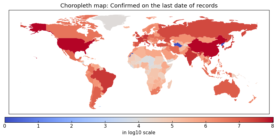
Additionally, we can create a choropleth map with a data at a geospatial layer on a date.
arguments of DataEngineer().choropleth():
geo (tuple(list[str] or tuple(str) or str) or str or None): location names to specify the layer or None (the top level)
variable (str): variable name to show
on (str or None): the date, like 22Jan2020, or None (the last date of each location)
title (str): title of the map
filename (str or None): filename to save the figure or None (display)
logscale (bool): whether convert the value to log10 scale values or not
directory (str): directory to save GeoJSON file of “Natural Earth” GitHub repository
natural_earth (str or None): title of GeoJSON file (without extension) of “Natural Earth” GitHub repository or None (automatically determined)
**kwargs: keyword arguments of the following classes and methods.
matplotlib.pyplot.savefig(), matplotlib.pyplot.legend(), and
pandas.DataFrame.plot()
[12]:
eng.choropleth(geo=None, variable="Confirmed", title="Choropleth map: Confirmed on the last date of records", filename=None)
5. Data subsetting for a location and data complement
The dataset is a geospatial time-series data. By selecting a location, the dataset will be converted to a time-series data, which is easier to analyze.
5.1 Subsetting
We will create a subset for selected location (eg. country, province/prefecture/state, city). Because the loaded dataset has country-level data, total values in United Kingdom (UK) on dates will be created here as an example.
Arguments of DataEngineer().subset():
geo (tuple(list[str] or tuple(str) or str) or str or None): location names to filter or None (total at the top level)
start_date (str or None): start date, like 22Jan2020
end_date (str or None): end date, like 01Feb2020
variables (list[str] or None): list of variables to add or None (all available columns)
complement (bool): whether perform data complement or not, True as default
get_dummies (bool): whether convert categorical variable into dummy variables or not, True as default
**Kwargs: keyword arguments for complement and default values
recovery_period (int): expected value of recovery period [days], 17
interval (int): expected update interval of the number of recovered cases [days], 2
max_ignored (int): Max number of recovered cases to be ignored [cases], 100
max_ending_unupdated (int): Max number of days to apply full complement, where max recovered cases are not updated [days], 14
upper_limit_days (int): maximum number of valid partial recovery periods [days], 90
lower_limit_days (int): minimum number of valid partial recovery periods [days], 7
upper_percentage (float): fraction of partial recovery periods with value greater than upper_limit_days, 0.5
lower_percentage (float): fraction of partial recovery periods with value less than lower_limit_days, 0.5
geo argument for subsetting when we have adequate data.When
geo=Noneorgeo=(None,), returns global scale records (total values of all country-level data), assuming we have country/province/city as layers here.When
geo=("Japan",)orgeo="Japan", returns country-level data in Japan.When
geo=(["Japan", "UK"],), returns country-level data of Japan and UK.When
geo=("Japan", "Tokyo"), returns province-level data of Tokyo/Japan.When
geo=("Japan", ["Tokyo", "Kanagawa"]), returns total values of province-level data of Tokyo/Japan and Kanagawa/Japan.When
geo=("Japan", "Kanagawa", "Yokohama"), returns city-level data of Yokohama/Kanagawa/Japan.When
geo=(("Japan", "Kanagawa", ["Yokohama", "Kawasaki"]), returns total values of city-level data of Yokohama/Kanagawa/Japan and Kawasaki/Kanagawa/Japan.
[13]:
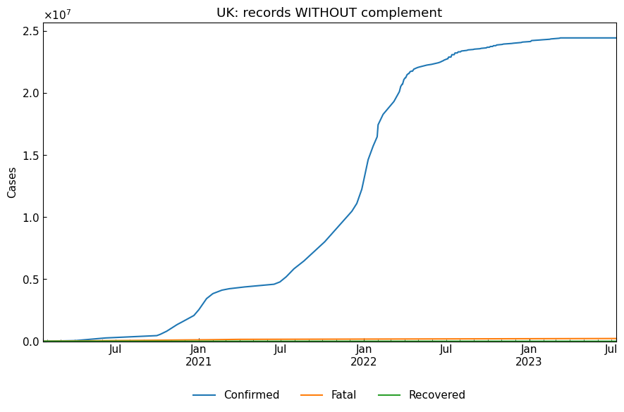
# Without complement
without_df, status, status_dict = eng.subset(geo="UK", complement=False)
print(f"{status}\n")
pprint(status_dict)
cs.line_plot(without_df[["Confirmed", "Fatal", "Recovered"]], title="UK: records WITHOUT complement")
{}
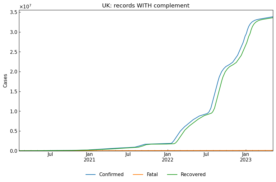
[14]:
# With complement (default)
with_df, status, status_dict = eng.subset(geo="Japan", complement=True)
print(f"{status}\n")
pprint(status_dict)
cs.line_plot(with_df[["Confirmed", "Fatal", "Recovered"]], title="UK: records WITH complement")
monotonic increasing complemented confirmed data and
monotonic increasing complemented fatal data and
fully complemented recovered data

{'Full_recovered': True,
 'Monotonic_confirmed': True,
 'Monotonic_fatal': True,
 'Monotonic_recovered': True,
 'Partial_recovered': False}
[15]:
with_df.info()
<class 'pandas.core.frame.DataFrame'>
DatetimeIndex: 1189 entries, 2020-02-05 to 2023-05-08
Data columns (total 32 columns):
 #   Column                                                         Non-Null Count  Dtype
---  ------                                                         --------------  -----
 0   Cancel_events                                                  1189 non-null   Float64
 1   Confirmed*Recovered                                            1189 non-null   Float64
 2   Confirmed_diff                                                 1189 non-null   Float64
 3   Contact_tracing                                                1189 non-null   Float64
 4   Fatal+Recovered                                                1189 non-null   Float64
 5   Gatherings_restrictions                                        1189 non-null   Float64
 6   Infected                                                       1189 non-null   Int64
 7   Information_campaigns                                          1189 non-null   Float64
 8   Internal_movement_restrictions                                 1189 non-null   Float64
 9   International_movement_restrictions                            1189 non-null   Float64
 10  Population                                                     1189 non-null   Float64
 11  Positive_rate                                                  1189 non-null   Float64
 12  Positive_rate_%                                                1189 non-null   Float64
 13  School_closing                                                 1189 non-null   Float64
 14  Stay_home_restrictions                                         1189 non-null   Float64
 15  Stringency_index                                               1189 non-null   Float64
 16  Susceptible                                                    1189 non-null   Float64
 17  Testing_policy                                                 1189 non-null   Float64
 18  Tests                                                          1189 non-null   Float64
 19  Transport_closing                                              1189 non-null   Float64
 20  Vaccinated_full                                                1189 non-null   Float64
 21  Vaccinated_once                                                1189 non-null   Float64
 22  Vaccinations                                                   1189 non-null   Float64
 23  Vaccinations_boosters                                          1189 non-null   Float64
 24  Workplace_closing                                              1189 non-null   Float64
 25  Confirmed                                                      1189 non-null   Int64
 26  Fatal                                                          1189 non-null   Int64
 27  Recovered                                                      1189 non-null   Int64
 28  Country_0                                                      1189 non-null   Int64
 29  Country_Japan                                                  1189 non-null   Int64
 30  Product_0                                                      1189 non-null   Int64
 31  Product_Moderna, Novavax, Oxford/AstraZeneca, Pfizer/BioNTech  1189 non-null   Int64
dtypes: Float64(24), Int64(8)
memory usage: 343.7 KB
5.2 Details of data complement
When complement=True (default), data complement will be performed for confirmed/fatal/recovered data. This may be required for analysis because reported cumulative values sometimes show decreasing by changing accidentally for an example. Additionally, some countries, including UK, do not report the number of recovered cases.
The possible kinds of complement for each country are the following:
“Monotonic_confirmed/fatal/recovered” (monotonic increasing complement) Force the variable show monotonic increasing.
“Full_recovered” (full complement of recovered data) Estimate the number of recovered cases using the value of estimated average recovery period.
“Partial_recovered” (partial complement of recovered data) When recovered values are not updated for some days, extrapolate the values.
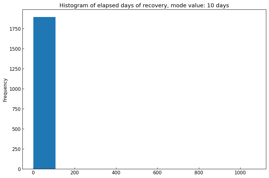
5.3 Recovery period
DataEngineer.recovery_period(data).[16]:
jpn_df, *_ = eng.subset(geo="Japan", variables=["Confirmed", "Fatal", "Recovered"], complement=False)
recovery_period = cs.DataEngineer.recovery_period(data=jpn_df)
print(f"Mode value of recovery period in Japan: {recovery_period} [days]")
Mode value of recovery period in Japan: 10 [days]
Details of recovery period calculation:
[17]:
df = jpn_df.resample("D").sum()
df["diff"] = df["Confirmed"] - df["Fatal"]
df = df.loc[:, ["diff", "Recovered"]].unstack().reset_index()
df.columns = ["Variable", "Date", "Number"]
df["Days"] = (df["Date"] - df["Date"].min()).dt.days
df = df.pivot_table(values="Days", index="Number", columns="Variable")
df = df.interpolate(limit_area="inside").dropna().astype(np.int64)
df["Elapsed"] = df["Recovered"] - df["diff"]
df = df.loc[df["Elapsed"] > 0]
# Calculate mode value
mode_value = round(df["Elapsed"].mode().mean())
df["Elapsed"].plot.hist(title=f"Histogram of elapsed days of recovery, mode value: {mode_value} days");
5.4 Alias of subsets
We can register alias names of subsets with DataEngineer().subset_alias().
Arguments:
alias (str or None): alias name or None (list-up alias names)
update (bool): force updating the alias when @alias is not None
**kwargs: keyword arguments of covsirphy.DataEngineer().subset()
[18]:
# Register
sub1, *_ = eng.subset_alias(alias="UK_with", geo="UK", complement=True)
# Retrieve with alias
sub2, *_ = eng.subset_alias(alias="UK_with")
# Comparison
sub1.equals(sub2)
[18]:
True
7. EDA of subset
With explanatory data analysis, we will get the figure of datasets.
7.1 Alias of variables
We can specify variables with alias. For example, “CIFR” is equivalent to list ['Confirmed', 'Infected', 'Recovered', 'Fatal'].
[19]:
eng.subset(geo="Japan", variables="CIRF")[0].tail()
[19]:
| Confirmed | Infected | Recovered | Fatal | |
|---|---|---|---|---|
| Date | ||||
| 2023-05-04 | 33791091 | 183209 | 33533260 | 74622 |
| 2023-05-05 | 33796902 | 177397 | 33544864 | 74641 |
| 2023-05-06 | 33803136 | 171546 | 33556937 | 74653 |
| 2023-05-07 | 33817576 | 175456 | 33567458 | 74662 |
| 2023-05-08 | 33826903 | 174762 | 33577464 | 74677 |
All aliases can be checked with DataEngineer().variables_alias().
[20]:
eng.variables_alias()
[20]:
{'N': ['Population'],
 'S': ['Susceptible'],
 'T': ['Tests'],
 'C': ['Confirmed'],
 'I': ['Infected'],
 'F': ['Fatal'],
 'R': ['Recovered'],
 'CFR': ['Confirmed', 'Fatal', 'Recovered'],
 'CIRF': ['Confirmed', 'Infected', 'Recovered', 'Fatal'],
 'SIRF': ['Susceptible', 'Infected', 'Recovered', 'Fatal'],
 'CR': ['Confirmed', 'Recovered']}
We can register new alias “p” with ["Tests", "Confirmed", "Positive_rate_%"] as an example.
[21]:
# Register new alias
eng.variables_alias(alias="p", variables=["Tests", "Confirmed", "Positive_rate_%"])
# Check the contents of an alias
eng.variables_alias(alias="p")
# Subsetting with the variable alias
eng.subset_alias(alias="jp", geo="Japan", variables="p")[0].tail()
[21]:
| Tests | Confirmed | Positive_rate_% | |
|---|---|---|---|
| Date | |||
| 2023-05-04 | 0.0 | 33791091 | inf |
| 2023-05-05 | 0.0 | 33796902 | inf |
| 2023-05-06 | 0.0 | 33803136 | inf |
| 2023-05-07 | 0.0 | 33817576 | inf |
| 2023-05-08 | 0.0 | 33826903 | inf |
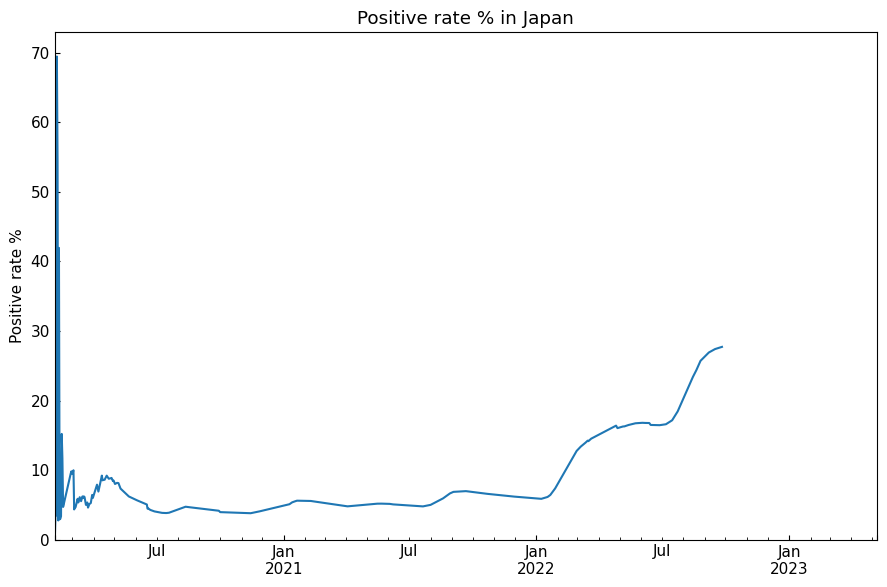
7.2 Line plot
Show data with line plot. We can select function line_plot or class LinePlot.
[22]:
line_df, *_ = eng.subset_alias(alias="jp")
With function:
[23]:
cs.line_plot(
    line_df["Positive_rate_%"],
    title="Positive rate % in Japan",
    ylabel="Positive rate %",
    math_scale=False,
    show_legend=False,
    filename=None,
)

With class:
[24]:
with cs.LinePlot(filename=None) as lp:
    lp.plot(line_df["Positive_rate_%"])
    lp.title = "Positive rate % in Japan"
    lp.x_axis(xlabel=None)
    lp.y_axis(ylabel="Positive rate %", math_scale=False)
    lp.legend_hide()
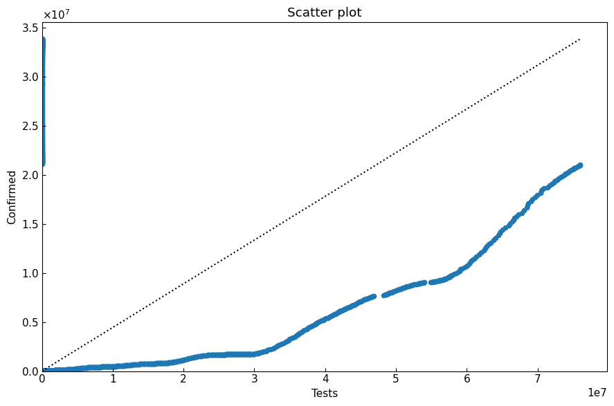
7.3 Scatter plot
Show data with scatter plot. We can select function scatter_plot or class ScatterPlot.
[25]:
sc_df, *_ = eng.subset_alias(alias="jp")
sc_df.rename(columns={"Tests": "x", "Confirmed": "y"}, inplace=True)
[26]:
cs.scatter_plot(
    sc_df,
    title="Scatter plot",
    xlabel="Tests", xlim=(0, None),
    ylabel="Confirmed",
    filename=None,
)
[27]:
with cs.ScatterPlot(filename=None) as sp:
    sp.plot(sc_df)
    sp.title = "Scatter plot"
    sp.x_axis(xlabel="Tests", xlim=(0, None))
    sp.y_axis(ylabel="Confirmed")
    sp.line_straight(p1=(0, 0), p2=(max(sc_df["x"]), max(sc_df["y"])))

Thank you!