![]()
Data preparation
The first step of data science is data preparation. covsirphy has the following three functionality for that.
Downloading datasets from recommended data servers
Reading
pandas.DataFrameGenerator of sample data with SIR-derived ODE model
[1]:
from datetime import date
from pprint import pprint
import numpy as np
import pandas as pd
import covsirphy as cs
cs.__version__
[1]:
'3.1.2.delta'
From version 2.28.0, some classes and methods output the following information using loguru: library which aims to bring enjoyable logging in Python. We can change logging level with cs.config(level=2) (as default).
level=0: errors (exceptions)level=1: errors, warningslevel=2: errors, warnings, info (start downloading/optimization)level=3: errors, warnings, info, debug
[2]:
cs.config.logger(level=2)
1. Downloading datasets from recommended data
We will download datasets from the following recommended data servers.
-
Guidotti, E., Ardia, D., (2020), “COVID-19 Data Hub”, Journal of Open Source Software 5(51):2376, doi: 10.21105/joss.02376.
The number of cases (JHU style)
Population values in each country/province
The number of tests
-
Hasell, J., Mathieu, E., Beltekian, D. et al. A cross-country database of COVID-19 testing. Sci Data 7, 345 (2020). https://doi.org/10.1038/s41597-020-00688-8
The number of tests
The number of vaccinations
The number of people who received vaccinations
COVID-19 Open Data by Google Cloud Platform
Wahltinez and others (2020), COVID-19 Open-Data: curating a fine-grained, global-scale data repository for SARS-CoV-2, Work in progress, https://goo.gle/covid-19-open-data
percentage to baseline in visits
Note: Please refer to Google Terms of Service in advance.
This will be removed because not updated. Refer to https://github.com/lisphilar/covid19-sir/issues/1224
World Population Prospects 2022
United Nations, Department of Economic and Social Affairs, Population Division (2022). World Population Prospects 2022, Online Edition.
Total population in each country
-
Hirokazu Takaya (2020-2022), GitHub repository, COVID-19 dataset in Japan, https://github.com/lisphilar/covid19-sir/tree/master/data
The number of cases in Japan (total/prefectures)
Metadata regarding Japan prefectures
1-1. With DataEngineer class
We can use DataEngineer().download() for data downloading from recommended data servers as the quickest way.
[3]:
eng = cs.DataEngineer()
eng.download(databases=["japan", "covid19dh", "owid"])
2025-12-15 at 13:30:18 | INFO | Retrieving COVID-19 dataset from https://github.com/lisphilar/covid19-sir/data/
2025-12-15 at 13:30:18 | INFO | Retrieving datasets from COVID-19 Data Hub https://covid19datahub.io/
2025-12-15 at 13:30:23 | INFO | Retrieving datasets from Our World In Data https://github.com/owid/covid-19-data/
2025-12-15 at 13:30:24 | INFO | Retrieving datasets from Our World In Data https://github.com/owid/covid-19-data/
2025-12-15 at 13:30:25 | INFO | Retrieving datasets from Our World In Data https://github.com/owid/covid-19-data/
[3]:
<covsirphy.engineering.engineer.DataEngineer at 0x7fd7c9450ef0>
We can get the all downloaded records as a pandas.DataFrame with DataEngineer().all() method.
[4]:
all_df = eng.all()
# Overview of the records
all_df.info()
<class 'pandas.core.frame.DataFrame'>
RangeIndex: 298052 entries, 0 to 298051
Data columns (total 27 columns):
 #   Column                               Non-Null Count   Dtype
---  ------                               --------------   -----
 0   ISO3                                 298052 non-null  category
 1   Province                             298052 non-null  category
 2   City                                 298052 non-null  category
 3   Date                                 298052 non-null  datetime64[ns]
 4   Cancel_events                        197839 non-null  Float64
 5   Confirmed                            239411 non-null  Float64
 6   Contact_tracing                      197865 non-null  Float64
 7   Country                              287385 non-null  string
 8   Fatal                                222214 non-null  Float64
 9   Gatherings_restrictions              197839 non-null  Float64
 10  Information_campaigns                197865 non-null  Float64
 11  Internal_movement_restrictions       197865 non-null  Float64
 12  International_movement_restrictions  197872 non-null  Float64
 13  Population                           286223 non-null  Float64
 14  Product                              176264 non-null  string
 15  Recovered                            74399 non-null   Float64
 16  School_closing                       197864 non-null  Float64
 17  Stay_home_restrictions               197833 non-null  Float64
 18  Stringency_index                     197828 non-null  Float64
 19  Testing_policy                       197865 non-null  Float64
 20  Tests                                91191 non-null   Float64
 21  Transport_closing                    197845 non-null  Float64
 22  Vaccinated_full                      59857 non-null   Float64
 23  Vaccinated_once                      62933 non-null   Float64
 24  Vaccinations                         66925 non-null   Float64
 25  Vaccinations_boosters                38050 non-null   Float64
 26  Workplace_closing                    197864 non-null  Float64
dtypes: Float64(21), category(3), datetime64[ns](1), string(2)
memory usage: 61.7 MB
DataEngineer.citations() shows citations of the datasets.
[5]:
print("\n".join(eng.citations()))
Hirokazu Takaya (2020-2024), COVID-19 dataset in Japan, GitHub repository, https://github.com/lisphilar/covid19-sir/data/japan
Guidotti, E., Ardia, D., (2020), "COVID-19 Data Hub", Journal of Open Source Software 5(51):2376, doi: 10.21105/joss.02376.
Hasell, J., Mathieu, E., Beltekian, D. et al. A cross-country database of COVID-19 testing. Sci Data 7, 345 (2020). https: //doi.org/10.1038/s41597-020-00688-8
Note that, as default, DataEngineer().download() collects country-level data and save the datasets as CSV files in “input” (=directory argument of DataEngineer().download()) folder of the current directory. If the last modification time of the saved CSV files is within the last 12 (=update_interval argument of DataEngineer().download()) hours, the saved CSV files will be used as the database.
For some countries (eg. Japan), province/state/prefecture level data is available and we can download it as follows.
[6]:
eng_jpn = cs.DataEngineer()
eng_jpn.download(country="Japan", databases=["japan", "covid19dh", "owid"])
eng_jpn.all().head()
2025-12-15 at 13:30:27 | INFO | Retrieving COVID-19 dataset from https://github.com/lisphilar/covid19-sir/data/
2025-12-15 at 13:30:28 | INFO | Retrieving datasets from COVID-19 Data Hub https://covid19datahub.io/
[6]:
| ISO3 | Province | City | Date | Cancel_events | Confirmed | Contact_tracing | Country | Fatal | Gatherings_restrictions | ... | Stay_home_restrictions | Stringency_index | Testing_policy | Tests | Transport_closing | Vaccinated_full | Vaccinated_once | Vaccinations | Vaccinations_boosters | Workplace_closing | |
|---|---|---|---|---|---|---|---|---|---|---|---|---|---|---|---|---|---|---|---|---|---|
| 0 | JPN | Aichi | - | 2020-03-18 | 1.0 | 130.0 | 2.0 | Japan | 14.0 | 0.0 | ... | 0.0 | -40.74 | 1.0 | 847.0 | 0.0 | None | None | None | None | 1.0 |
| 1 | JPN | Aichi | - | 2020-03-19 | 1.0 | 134.0 | 2.0 | Japan | 14.0 | 0.0 | ... | 0.0 | -40.74 | 1.0 | 847.0 | 0.0 | None | None | None | None | 1.0 |
| 2 | JPN | Aichi | - | 2020-03-20 | 1.0 | 139.0 | 2.0 | Japan | 16.0 | 0.0 | ... | 0.0 | -40.74 | 1.0 | 847.0 | 0.0 | None | None | None | None | 1.0 |
| 3 | JPN | Aichi | - | 2020-03-21 | 1.0 | 141.0 | 2.0 | Japan | 16.0 | 0.0 | ... | 0.0 | -40.74 | 1.0 | 847.0 | 0.0 | None | None | None | None | 1.0 |
| 4 | JPN | Aichi | - | 2020-03-22 | 1.0 | 143.0 | 2.0 | Japan | 16.0 | 0.0 | ... | 0.0 | -40.74 | 1.0 | 847.0 | 0.0 | None | None | None | None | 1.0 |
5 rows × 26 columns
For some countries (eg. USA), city-level data is available and we can download it as follows.
[7]:
eng_alabama = cs.DataEngineer()
eng_alabama.download(country="USA", province="Alabama", databases=["japan", "covid19dh", "owid"])
eng_alabama.all().head()
2025-12-15 at 13:30:29 | INFO | Retrieving datasets from COVID-19 Data Hub https://covid19datahub.io/
[7]:
| ISO3 | Province | City | Date | Cancel_events | Confirmed | Contact_tracing | Country | Fatal | Gatherings_restrictions | ... | International_movement_restrictions | Population | Recovered | School_closing | Stay_home_restrictions | Stringency_index | Testing_policy | Tests | Transport_closing | Workplace_closing | |
|---|---|---|---|---|---|---|---|---|---|---|---|---|---|---|---|---|---|---|---|---|---|
| 0 | USA | Alabama | Autauga | 2020-03-24 | -2.0 | 1.0 | 1.0 | United States | 0.0 | -4.0 | ... | 3.0 | 55869.0 | <NA> | 3.0 | -2.0 | -68.98 | 1.0 | <NA> | -1.0 | -3.0 |
| 1 | USA | Alabama | Autauga | 2020-03-25 | -2.0 | 4.0 | 1.0 | United States | 0.0 | -4.0 | ... | 3.0 | 55869.0 | <NA> | 3.0 | -2.0 | -68.98 | 1.0 | <NA> | -1.0 | -3.0 |
| 2 | USA | Alabama | Autauga | 2020-03-26 | -2.0 | 6.0 | 1.0 | United States | 0.0 | -4.0 | ... | 3.0 | 55869.0 | <NA> | 3.0 | -2.0 | -68.98 | 1.0 | <NA> | -1.0 | -3.0 |
| 3 | USA | Alabama | Autauga | 2020-03-27 | -2.0 | 6.0 | 1.0 | United States | 0.0 | -4.0 | ... | 3.0 | 55869.0 | <NA> | 3.0 | -2.0 | -68.98 | 1.0 | <NA> | -1.0 | -3.0 |
| 4 | USA | Alabama | Autauga | 2020-03-28 | 2.0 | 6.0 | 1.0 | United States | 0.0 | -4.0 | ... | 3.0 | 55869.0 | <NA> | 3.0 | -2.0 | -73.61 | 1.0 | <NA> | -1.0 | 3.0 |
5 rows × 22 columns
Move forward to Tutorial: Data engineering.
1-2. With DataDownloader class
DataEngineer class is useful because it has data cleaning methods and so on (explained with Tutorial: Data engineering), but we can use DataDownloader class for data downloading.
[8]:
dl = cs.DataDownloader()
dl_df = dl.layer(country=None, province=None, databases=["japan", "covid19dh", "owid"])
[9]:
# Overview of the records
dl_df.info()
<class 'pandas.core.frame.DataFrame'>
RangeIndex: 298052 entries, 0 to 298051
Data columns (total 27 columns):
 #   Column                               Non-Null Count   Dtype
---  ------                               --------------   -----
 0   ISO3                                 298052 non-null  string
 1   Province                             298052 non-null  string
 2   City                                 298052 non-null  string
 3   Date                                 298052 non-null  datetime64[ns]
 4   Cancel_events                        197839 non-null  Int64
 5   Confirmed                            239411 non-null  Float64
 6   Contact_tracing                      197865 non-null  Int64
 7   Country                              287385 non-null  string
 8   Fatal                                222214 non-null  Float64
 9   Gatherings_restrictions              197839 non-null  Int64
 10  Information_campaigns                197865 non-null  Int64
 11  Internal_movement_restrictions       197865 non-null  Int64
 12  International_movement_restrictions  197872 non-null  Int64
 13  Population                           286223 non-null  Int64
 14  Product                              176264 non-null  string
 15  Recovered                            74399 non-null   Float64
 16  School_closing                       197864 non-null  Int64
 17  Stay_home_restrictions               197833 non-null  Int64
 18  Stringency_index                     197828 non-null  Float64
 19  Testing_policy                       197865 non-null  Int64
 20  Tests                                91191 non-null   Float64
 21  Transport_closing                    197845 non-null  Int64
 22  Vaccinated_full                      59857 non-null   Float64
 23  Vaccinated_once                      62933 non-null   Float64
 24  Vaccinations                         66925 non-null   Float64
 25  Vaccinations_boosters                38050 non-null   Float64
 26  Workplace_closing                    197864 non-null  Int64
dtypes: Float64(9), Int64(12), datetime64[ns](1), string(5)
memory usage: 67.4 MB
Note that ISO3/Province/City columns have string data instead of categorical data.
[10]:
# Citations
print("\n".join(dl.citations()))
Hirokazu Takaya (2020-2024), COVID-19 dataset in Japan, GitHub repository, https://github.com/lisphilar/covid19-sir/data/japan
Guidotti, E., Ardia, D., (2020), "COVID-19 Data Hub", Journal of Open Source Software 5(51):2376, doi: 10.21105/joss.02376.
Hasell, J., Mathieu, E., Beltekian, D. et al. A cross-country database of COVID-19 testing. Sci Data 7, 345 (2020). https: //doi.org/10.1038/s41597-020-00688-8
Acknowledgement
In Feb2020, CovsirPhy project started in Kaggle platform with COVID-19 data with SIR model notebook by Hirokazu Takaya helped by Kagglers using the following datasets.
The number of cases (JHU) and linelist: Novel Corona Virus 2019 Dataset by SRK
Population in each country: covid19 global forecasting: locations population by Dmitry A. Grechka
The number of cases in Japan: COVID-19 dataset in Japan by Lisphilar
The current version of covsirphy does not have interfaces to use the datasets in Kaggle because they are not updated at this time. However, we could not have done CovsirPhy project without their supports. Thank you!!
2. Reading pandas.DataFrame
We may need to use our own datasets for analysis because the dataset is not included in the recommended data servers. DataEngineer().register() registers new datasets of pandas.DataFrame format.
2-1. Retrieve Monkeypox line list
At first, we will prepare the new dataset as pandas.DataFrame. We will use Global.health Monkeypox under CC BY 4.0 license, line list data regarding Monkeypox 2022, just for demonstration.
[11]:
today = date.today()
mp_cite = f"Global.health Monkeypox (accessed on {today.strftime('%Y-%m-%d')}):\n" \
    "Kraemer, Tegally, Pigott, Dasgupta, Sheldon, Wilkinson, Schultheiss, et al. " \
    "Tracking the 2022 Monkeypox Outbreak with Epidemiological Data in Real-Time. " \
    "The Lancet Infectious Diseases. https://doi.org/10.1016/S1473-3099(22)00359-0.\n" \
    "European Centre for Disease Prevention and Control/WHO Regional Office for Europe." \
    f" Monkeypox, Joint Epidemiological overview, {today.day} {today.month}, 2022"
print(mp_cite)
Global.health Monkeypox (accessed on 2025-12-15):
Kraemer, Tegally, Pigott, Dasgupta, Sheldon, Wilkinson, Schultheiss, et al. Tracking the 2022 Monkeypox Outbreak with Epidemiological Data in Real-Time. The Lancet Infectious Diseases. https://doi.org/10.1016/S1473-3099(22)00359-0.
European Centre for Disease Prevention and Control/WHO Regional Office for Europe. Monkeypox, Joint Epidemiological overview, 15 12, 2022
Retrieve CSV file with pandas.read_csv(), using Pyarrow as the engine.
[12]:
# Deprecated: Final line list from Global.health, as of 2022-09-22
raw_url = "https://raw.githubusercontent.com/globaldothealth/monkeypox/9035dfb1303c05c380f86a3c1e00f81a1cc4046b/latest_deprecated.csv"
raw = pd.read_csv(raw_url, engine="pyarrow")
raw.info()
<class 'pandas.core.frame.DataFrame'>
RangeIndex: 69595 entries, 0 to 69594
Data columns (total 36 columns):
 #   Column                   Non-Null Count  Dtype
---  ------                   --------------  -----
 0   ID                       69595 non-null  object
 1   Status                   69595 non-null  object
 2   Location                 52387 non-null  object
 3   City                     1383 non-null   object
 4   Country                  69595 non-null  object
 5   Country_ISO3             69595 non-null  object
 6   Age                      3021 non-null   object
 7   Gender                   2475 non-null   object
 8   Date_onset               77 non-null     object
 9   Date_confirmation        65546 non-null  object
 10  Symptoms                 220 non-null    object
 11  Hospitalised (Y/N/NA)    354 non-null    object
 12  Date_hospitalisation     35 non-null     object
 13  Isolated (Y/N/NA)        493 non-null    object
 14  Date_isolation           16 non-null     object
 15  Outcome                  101 non-null    object
 16  Contact_comment          91 non-null     object
 17  Contact_ID               27 non-null     float64
 18  Contact_location         6 non-null      object
 19  Travel_history (Y/N/NA)  365 non-null    object
 20  Travel_history_entry     42 non-null     object
 21  Travel_history_start     11 non-null     object
 22  Travel_history_location  114 non-null    object
 23  Travel_history_country   99 non-null     object
 24  Genomics_Metadata        24 non-null     object
 25  Confirmation_method      100 non-null    object
 26  Source                   69595 non-null  object
 27  Source_II                8240 non-null   object
 28  Source_III               893 non-null    object
 29  Source_IV                54 non-null     object
 30  Source_V                 0 non-null      float64
 31  Source_VI                0 non-null      float64
 32  Source_VII               0 non-null      float64
 33  Date_entry               69595 non-null  object
 34  Date_death               83 non-null     object
 35  Date_last_modified       69595 non-null  object
dtypes: float64(4), object(32)
memory usage: 19.1+ MB
Review the data.
[13]:
raw.head()
[13]:
| ID | Status | Location | City | Country | Country_ISO3 | Age | Gender | Date_onset | Date_confirmation | ... | Source | Source_II | Source_III | Source_IV | Source_V | Source_VI | Source_VII | Date_entry | Date_death | Date_last_modified | |
|---|---|---|---|---|---|---|---|---|---|---|---|---|---|---|---|---|---|---|---|---|---|
| 0 | N1 | confirmed | Guy's and St Thomas Hospital London | London | England | GBR | None | None | 2022-04-29 | 2022-05-06 | ... | https://www.gov.uk/government/news/monkeypox-c... | https://www.who.int/emergencies/disease-outbre... | None | None | NaN | NaN | NaN | 2022-05-18 | None | 2022-05-18 |
| 1 | N2 | confirmed | Guy's and St Thomas Hospital London | London | England | GBR | None | None | 2022-05-05 | 2022-05-12 | ... | https://www.gov.uk/government/news/monkeypox-c... | None | None | None | NaN | NaN | NaN | 2022-05-18 | None | 2022-05-18 |
| 2 | N3 | confirmed | London | London | England | GBR | None | None | 2022-04-30 | 2022-05-13 | ... | https://www.gov.uk/government/news/monkeypox-c... | None | None | None | NaN | NaN | NaN | 2022-05-18 | None | 2022-05-18 |
| 3 | N4 | confirmed | London | London | England | GBR | None | male | None | 2022-05-15 | ... | https://www.gov.uk/government/news/monkeypox-c... | None | None | None | NaN | NaN | NaN | 2022-05-18 | None | 2022-05-18 |
| 4 | N5 | confirmed | London | London | England | GBR | None | male | None | 2022-05-15 | ... | https://www.gov.uk/government/news/monkeypox-c... | None | None | None | NaN | NaN | NaN | 2022-05-18 | None | 2022-05-18 |
5 rows × 36 columns
[14]:
pprint(raw.Status.unique())
pprint(raw.Outcome.unique())
array(['confirmed', 'discarded', 'suspected', 'omit_error'], dtype=object)
array([None, 'Recovered', 'Death'], dtype=object)
2-2. Convert line list to the number of cases data
Prepare analyzable data, converting the line list to the number of cases. This step may be skipped because we have datasets with the number of cases.
Prepare PPT (per protocol set) data.
[15]:
date_cols = [
    "Date_onset", "Date_confirmation", "Date_hospitalisation",
    "Date_isolation", "Date_death", "Date_last_modified"
]
cols = ["ID", "Status", "City", "Country_ISO3", "Outcome", *date_cols]
df = raw.loc[:, cols].rename(columns={"Country_ISO3": "ISO3"})
df = df.loc[df["Status"].isin(["confirmed", "suspected"])]

for col in date_cols:
    df[col] = pd.to_datetime(df[col])

df["Date_min"] = df[date_cols].min(axis=1)
df["Date_recovered"] = df[["Outcome", "Date_last_modified"]].apply(
    lambda x: x[1] if x[0] == "Recovered" else pd.NaT, axis=1)
df["City"] = df["City"].replace('', pd.NA).fillna("Unknown")

ppt_df = df.copy()
ppt_df.head()
[15]:
| ID | Status | City | ISO3 | Outcome | Date_onset | Date_confirmation | Date_hospitalisation | Date_isolation | Date_death | Date_last_modified | Date_min | Date_recovered | |
|---|---|---|---|---|---|---|---|---|---|---|---|---|---|
| 0 | N1 | confirmed | London | GBR | None | 2022-04-29 | 2022-05-06 | 2022-05-04 | 2022-05-04 | NaT | 2022-05-18 | 2022-04-29 | NaT |
| 1 | N2 | confirmed | London | GBR | None | 2022-05-05 | 2022-05-12 | 2022-05-06 | 2022-05-09 | NaT | 2022-05-18 | 2022-05-05 | NaT |
| 2 | N3 | confirmed | London | GBR | None | 2022-04-30 | 2022-05-13 | NaT | NaT | NaT | 2022-05-18 | 2022-04-30 | NaT |
| 3 | N4 | confirmed | London | GBR | None | NaT | 2022-05-15 | NaT | NaT | NaT | 2022-05-18 | 2022-05-15 | NaT |
| 4 | N5 | confirmed | London | GBR | None | NaT | 2022-05-15 | NaT | NaT | NaT | 2022-05-18 | 2022-05-15 | NaT |
Calculate daily new confirmed cases.
[16]:
df = ppt_df.rename(columns={"Date_min": "Date"})
series = df.groupby(["ISO3", "City", "Date"])["ID"].count()
series.name = "Confirmed"
c_df = pd.DataFrame(series)
c_df.head()
[16]:
| Confirmed | |||
|---|---|---|---|
| ISO3 | City | Date | |
| ABW | Unknown | 2022-08-22 | 1 |
| 2022-08-29 | 1 | ||
| 2022-09-13 | 1 | ||
| AND | Unknown | 2022-07-25 | 1 |
| 2022-07-26 | 2 |
Calculate daily new recovered cases.
[17]:
df = ppt_df.rename(columns={"Date_recovered": "Date"})
series = df.groupby(["ISO3", "City", "Date"])["ID"].count()
series.name = "Recovered"
r_df = pd.DataFrame(series)
r_df.head()
[17]:
| Recovered | |||
|---|---|---|---|
| ISO3 | City | Date | |
| AUS | Melbourne | 2022-06-30 | 1 |
| TUR | Unknown | 2022-08-05 | 4 |
Calculate daily new fatal cases.
[18]:
df = ppt_df.rename(columns={"Date_death": "Date"})
series = df.groupby(["ISO3", "City", "Date"])["ID"].count()
series.name = "Fatal"
f_df = pd.DataFrame(series)
f_df.head()
[18]:
| Fatal | |||
|---|---|---|---|
| ISO3 | City | Date | |
| BEL | Unknown | 2022-08-29 | 1 |
| BRA | Unknown | 2022-07-28 | 1 |
| 2022-08-29 | 1 | ||
| CAF | Unknown | 2022-03-04 | 2 |
| COD | Unknown | 2022-01-16 | 18 |
Combine data (cumulative number).
[19]:
df = c_df.combine_first(f_df).combine_first(r_df)
df = df.unstack(level=["ISO3", "City"])
df = df.asfreq("D").fillna(0).cumsum()
df = df.stack(level=["ISO3", "City"]).reorder_levels(["ISO3", "City", "Date"])
df = df.sort_index().reset_index()
all_df_city = df.copy()
all_df_city.head()
[19]:
| ISO3 | City | Date | Confirmed | Fatal | Recovered | |
|---|---|---|---|---|---|---|
| 0 | ABW | Unknown | 2022-01-16 | 0.0 | 0.0 | 0.0 |
| 1 | ABW | Unknown | 2022-01-17 | 0.0 | 0.0 | 0.0 |
| 2 | ABW | Unknown | 2022-01-18 | 0.0 | 0.0 | 0.0 |
| 3 | ABW | Unknown | 2022-01-19 | 0.0 | 0.0 | 0.0 |
| 4 | ABW | Unknown | 2022-01-20 | 0.0 | 0.0 | 0.0 |
At country level (City = “-”) and city level (City != “-“):
[20]:
df2 = all_df_city.groupby(["ISO3", "Date"], as_index=False).sum()
df2["City"] = "-"
df = pd.concat([df2, all_df_city], axis=0)
df = df.loc[df["City"] != "Unknown"]
all_df = df.convert_dtypes()
all_df
[20]:
| ISO3 | Date | City | Confirmed | Fatal | Recovered | |
|---|---|---|---|---|---|---|
| 0 | ABW | 2022-01-16 | - | 0 | 0 | 0 |
| 1 | ABW | 2022-01-17 | - | 0 | 0 | 0 |
| 2 | ABW | 2022-01-18 | - | 0 | 0 | 0 |
| 3 | ABW | 2022-01-19 | - | 0 | 0 | 0 |
| 4 | ABW | 2022-01-20 | - | 0 | 0 | 0 |
| ... | ... | ... | ... | ... | ... | ... |
| 69245 | ZAF | 2022-09-18 | Johannesburg | 1 | 0 | 0 |
| 69246 | ZAF | 2022-09-19 | Johannesburg | 1 | 0 | 0 |
| 69247 | ZAF | 2022-09-20 | Johannesburg | 1 | 0 | 0 |
| 69248 | ZAF | 2022-09-21 | Johannesburg | 1 | 0 | 0 |
| 69249 | ZAF | 2022-09-22 | Johannesburg | 1 | 0 | 0 |
70500 rows × 6 columns
Check data.
[21]:
gis = cs.GIS(layers=["ISO3", "City"], country="ISO3", date="Date")
gis.register(data=all_df, convert_iso3=False);
[22]:
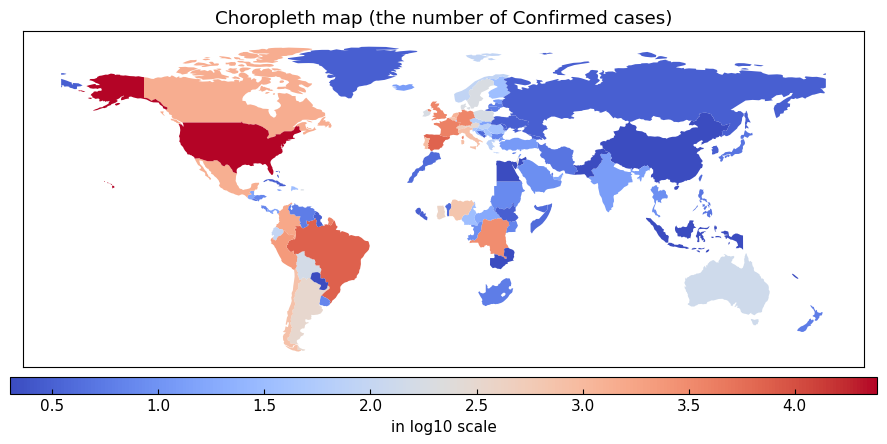
variable = "Confirmed"
gis.choropleth(
    variable=variable, filename=None,
    title=f"Choropleth map (the number of {variable} cases)"
)
2025-12-15 at 13:31:17 | INFO | Retrieving GIS data from Natural Earth https://www.naturalearthdata.com/
[23]:
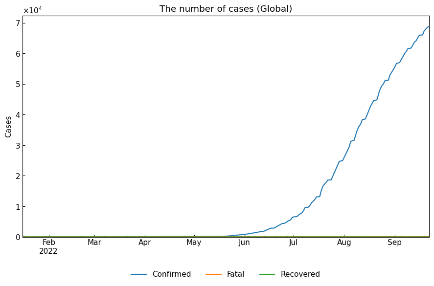
global_df = gis.subset(geo=None).set_index("Date").astype(np.int64)
global_df.tail()
cs.line_plot(global_df, title="The number of cases (Global)")
2-3. Retrieve total population data
So that we can analyze the data, total population values are necessary (we will confirm this with Tutorial: SIR-derived ODE models later).
Population data at country-level can be retrieved with DataDownloader().layer(databases=["wpp"]) via DataEngineer().register(databases=["wpp"]).
[24]:
# Set layers and specify layer name of country
# (which will be converted to ISO3 code for standardization)
eng = cs.DataEngineer(layers=["ISO3", "City"], country=["ISO3"])
# Download and automated registration of population data
eng.download(databases=["wpp"])
# Specify date range to reduce the memory
date_range = (all_df["Date"].min(), all_df["Date"].max())
eng.clean(kinds=["resample"], date_range=date_range)
# Show all data
display(eng.all())
# Show citations
pprint(eng.citations())
2025-12-15 at 13:31:20 | INFO | [INFO] 'Province' layer was removed.
| ISO3 | City | Date | Population | |
|---|---|---|---|---|
| 0 | ABW | - | 2022-07-01 | 107310.0 |
| 1 | AFE | - | 2022-07-01 | 731821393.0 |
| 2 | AFG | - | 2022-07-01 | 40578842.0 |
| 3 | AFW | - | 2022-07-01 | 497387180.0 |
| 4 | AGO | - | 2022-07-01 | 35635029.0 |
| ... | ... | ... | ... | ... |
| 256 | XKX | - | 2022-07-01 | 1768096.0 |
| 257 | YEM | - | 2022-07-01 | 38222876.0 |
| 258 | ZAF | - | 2022-07-01 | 62378410.0 |
| 259 | ZMB | - | 2022-07-01 | 20152938.0 |
| 260 | ZWE | - | 2022-07-01 | 16069056.0 |
261 rows × 4 columns
['United Nations, Department of Economic and Social Affairs, Population '
 'Division (2022). World Population Prospects 2022, Online Edition.']
2-4. Register Monkeypox data
Register the Monkeypox data to DataEngineer() instance.
[25]:
eng.register(data=all_df, citations=[mp_cite])
# Show all data
display(eng.all())
# Show citations
pprint(eng.citations())
| ISO3 | City | Date | Confirmed | Fatal | Population | Recovered | |
|---|---|---|---|---|---|---|---|
| 0 | ABW | - | 2022-01-16 | 0 | 0 | <NA> | 0 |
| 1 | ABW | - | 2022-01-17 | 0 | 0 | <NA> | 0 |
| 2 | ABW | - | 2022-01-18 | 0 | 0 | <NA> | 0 |
| 3 | ABW | - | 2022-01-19 | 0 | 0 | <NA> | 0 |
| 4 | ABW | - | 2022-01-20 | 0 | 0 | <NA> | 0 |
| ... | ... | ... | ... | ... | ... | ... | ... |
| 70644 | ZMB | - | 2022-09-19 | 1 | 0 | <NA> | 0 |
| 70645 | ZMB | - | 2022-09-20 | 1 | 0 | <NA> | 0 |
| 70646 | ZMB | - | 2022-09-21 | 1 | 0 | <NA> | 0 |
| 70647 | ZMB | - | 2022-09-22 | 1 | 0 | <NA> | 0 |
| 70648 | ZWE | - | 2022-07-01 | <NA> | <NA> | 16069056.0 | <NA> |
70649 rows × 7 columns
['United Nations, Department of Economic and Social Affairs, Population '
 'Division (2022). World Population Prospects 2022, Online Edition.',
 'Global.health Monkeypox (accessed on 2025-12-15):\n'
 'Kraemer, Tegally, Pigott, Dasgupta, Sheldon, Wilkinson, Schultheiss, et al. '
 'Tracking the 2022 Monkeypox Outbreak with Epidemiological Data in Real-Time. '
 'The Lancet Infectious Diseases. '
 'https://doi.org/10.1016/S1473-3099(22)00359-0.\n'
 'European Centre for Disease Prevention and Control/WHO Regional Office for '
 'Europe. Monkeypox, Joint Epidemiological overview, 15 12, 2022']
Move forward to Tutorial: Data engineering.
3. Generator of sample data with SIR-derived ODE model
CovsirPhy can generate sample data with subclasses of ODEModel and Dynamics class. Refer to the followings.
3.1 Sample data of one-phase ODE model
Regarding ODE models, please refer to Tutorial: SIR-derived ODE models. Here, we will create a sample data with one-phase SIR model and tau value 1440 min, the first date 01Jan2022, the last date 30Jun2022. ODE parameter values are preset.
[26]:
# Create solver with preset
model = cs.SIRModel.from_sample(date_range=("01Jan2022", "30Jun2022"), tau=1440)
# Show settings
pprint(model.settings())
{'date_range': ('01Jan2022', '30Jun2022'),
 'initial_dict': {'Fatal or Recovered': 0,
                  'Infected': 1000,
                  'Susceptible': 999000},
 'param_dict': {'rho': 0.2, 'sigma': 0.075},
 'tau': 1440}
Solve the ODE model with ODEModel().solve() method.
[27]:
one_df = model.solve()
display(one_df.head())
display(one_df.tail())
| Susceptible | Infected | Fatal or Recovered | |
|---|---|---|---|
| Date | |||
| 2022-01-01 | 999000 | 1000 | 0 |
| 2022-01-02 | 998787 | 1133 | 80 |
| 2022-01-03 | 998546 | 1283 | 170 |
| 2022-01-04 | 998273 | 1454 | 273 |
| 2022-01-05 | 997964 | 1647 | 389 |
| Susceptible | Infected | Fatal or Recovered | |
|---|---|---|---|
| Date | |||
| 2022-06-26 | 88354 | 750 | 910895 |
| 2022-06-27 | 88342 | 708 | 910950 |
| 2022-06-28 | 88329 | 669 | 911002 |
| 2022-06-29 | 88318 | 632 | 911050 |
| 2022-06-30 | 88307 | 596 | 911096 |
Plot the time-series data.
[28]:
cs.line_plot(one_df, title=f"Sample data of SIR model {model.settings()['param_dict']}")
3.2 Sample data of multi-phase ODE model
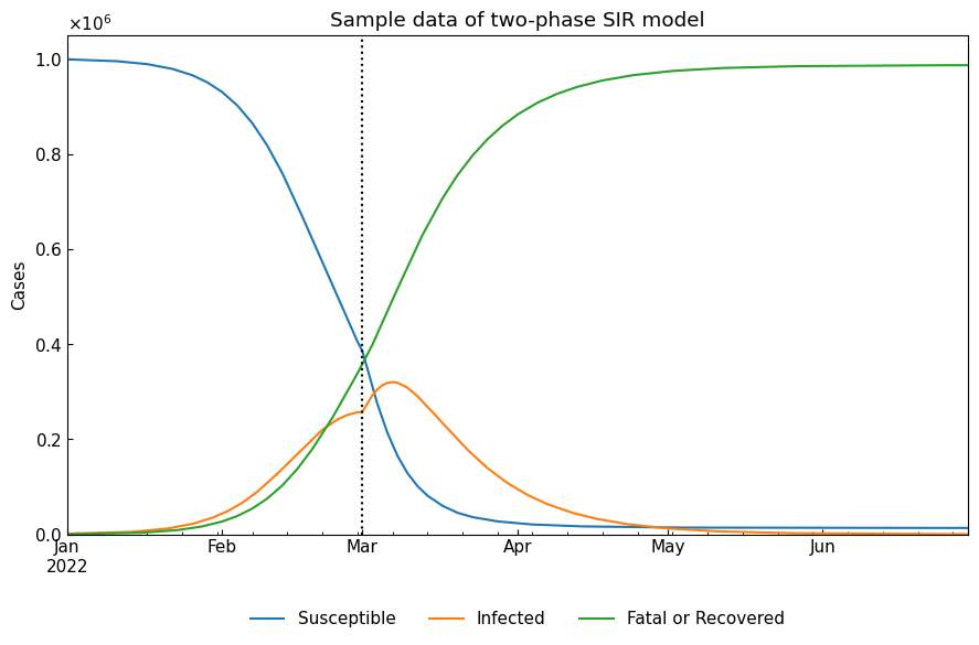
Regarding multi-phase ODE models, please refer to Phase-dependent SIR models. Here, we will create a sample data with two-phase SIR model and tau value 1440 min, the first date 01Jan2022, the last date 30Jun2022.
We will use Dynamics class. At first, set the first/date of dynamics and set th 0th phase ODE parameters.
[29]:
dyn = cs.Dynamics.from_sample(model=cs.SIRModel, date_range=("01Jan2022", "30Jun2022"))
# Show summary
dyn.summary()
[29]:
| Start | End | Rt | rho | sigma | 1/beta [day] | 1/gamma [day] | |
|---|---|---|---|---|---|---|---|
| Phase | |||||||
| 0th | 2022-01-01 | 2022-06-30 | 2.67 | 0.2 | 0.075 | 5 | 13 |
Add the 1st phase with Dynamics.register() method.
[30]:
setting_df = dyn.register()
setting_df.loc["01Mar2022": "30Jun2022", ["rho", "sigma"]] = [0.4, 0.075]
setting_df
[30]:
| Susceptible | Infected | Recovered | Fatal | rho | sigma | |
|---|---|---|---|---|---|---|
| Date | ||||||
| 2022-01-01 | 999000.0 | 1000.0 | 0.0 | 0.0 | 0.2 | 0.075 |
| 2022-01-02 | <NA> | <NA> | <NA> | <NA> | <NA> | <NA> |
| 2022-01-03 | <NA> | <NA> | <NA> | <NA> | <NA> | <NA> |
| 2022-01-04 | <NA> | <NA> | <NA> | <NA> | <NA> | <NA> |
| 2022-01-05 | <NA> | <NA> | <NA> | <NA> | <NA> | <NA> |
| ... | ... | ... | ... | ... | ... | ... |
| 2022-06-26 | <NA> | <NA> | <NA> | <NA> | 0.4 | 0.075 |
| 2022-06-27 | <NA> | <NA> | <NA> | <NA> | 0.4 | 0.075 |
| 2022-06-28 | <NA> | <NA> | <NA> | <NA> | 0.4 | 0.075 |
| 2022-06-29 | <NA> | <NA> | <NA> | <NA> | 0.4 | 0.075 |
| 2022-06-30 | <NA> | <NA> | <NA> | <NA> | 0.4 | 0.075 |
181 rows × 6 columns
[31]:
dyn.register(data=setting_df)
# Show summary
dyn.summary()
[31]:
| Start | End | Rt | rho | sigma | 1/beta [day] | 1/gamma [day] | |
|---|---|---|---|---|---|---|---|
| Phase | |||||||
| 0th | 2022-01-01 | 2022-02-28 | 2.67 | 0.2 | 0.075 | 5 | 13 |
| 1st | 2022-03-01 | 2022-06-30 | 5.33 | 0.4 | 0.075 | 2 | 13 |
Solve the ODE model with Dynamics().simulate() method and plot the time-series data.
[32]:
two_df = dyn.simulate(model_specific=True)
cs.line_plot(two_df, title="Sample data of two-phase SIR model", v=["01Mar2022"])
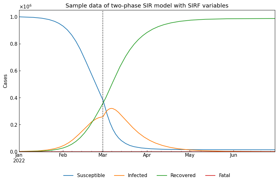
When we need convert model-specific variables to model-free variables (Susceptible/Infected/Fatal/Recovered), we will set model_specific=False (default). Because R=”Fatal or Recovered” in SIR model, we assume that R=”Recovered” and F = 0.
[33]:
two_df = dyn.simulate(model_specific=False)
cs.line_plot(two_df, title="Sample data of two-phase SIR model with SIRF variables", v=["01Mar2022"])
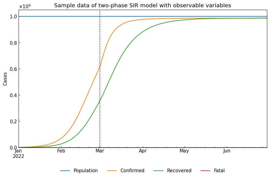
Actually, observable variables are Population/Confirmed/Infected/Recovered. We can calculate Population and Confirmed as follows.
Confirmed = Infected + Fatal + Recovered
Population = Susceptible + Confirmed
[34]:
real_df = two_df.copy()
real_df["Confirmed"] = real_df[["Infected", "Fatal", "Recovered"]].sum(axis=1)
real_df["Population"] = real_df[["Susceptible", "Confirmed"]].sum(axis=1)
real_df = real_df.loc[:, ["Population", "Confirmed", "Recovered", "Fatal"]]
cs.line_plot(real_df, title="Sample data of two-phase SIR model with observable variables", v=["01Mar2022"])
Thank you!